Hot Take Alert

Jonathan Taylor is on pace to be the greatest running back in Wisconsin football history.

Over the previous three decades Wisconsin has retained several elite rushers (and offensive lines) to amass several conference championships and Rose Bowl appearances. Even when acknowledging Taylor’s case as a serious Heisman candidate in each of his first two years, proclaiming him the presumptive best running back in Wisconsin football history still feels like a bold proclamation. Let’s investigate!

Accessing the data

The first step in comparing Taylor to previous Wisconsin rushers is retrieving historical college football statistics. Single-game box scores are only available on Sports-Reference starting in 2000 (compare the game hyperlinks for the 1999 and 2000 Wisconsin schedules), therefore, two scripts were used to aggregate player data:

The first accesses single season statistics from 1956-2018, detailed here (NOTE: click on the ▶ details to display the code!)

Scraper for Yearly Rushing Data, 1956 - 2018

    library(dplyr)
    library(rvest)
    library(ggplot2)
    library(lubridate)
    library(shadowtext)
    library(RColorBrewer)
    library(ggrepel)
    library(forcats)

    url <- "https://www.sports-reference.com/cfb/schools/wisconsin/"

    rushingTable <- '#rushing_and_receiving'
    playerIDTable <- paste0(rushingTable,' a')
    rushingData <- data.frame()

# for loop by season
    for (season in 1956:1999) {
      html <- paste0(url,season,".html")

#   batting stats
      html %>%
        read_html %>%
        html_nodes(xpath = '//comment()') %>%
        html_text() %>%
        paste(collapse='') %>%
        read_html() %>%
        html_node(rushingTable) %>%
        html_table(header = TRUE) -> df

#   player info
      html %>%
        read_html %>%
        html_nodes(xpath = '//comment()') %>%
        html_text() %>%
        paste(collapse='') %>%
        read_html() %>%
        html_nodes(playerIDTable) %>%
        html_attr(name="href") %>% unlist %>% as.character -> playerIDhtml

#   clean dataframe and add team and season info
      colnames(df) <- df[1,]
      df <- df[-1, ]
      df$season <- c(season)

 #  remove url data
      playerIDhtml=gsub("/cfb/players/", "", playerIDhtml,fixed = TRUE)
      playerID=gsub(".html", "", playerIDhtml,fixed = TRUE)

      df$playerID <- c(playerID)

#   bind to
      rushingData <- rbind(rushingData,df)
    }

The second accesses single game statistics from 2000-2018.

Scraper for Single Game Rushing Data, 2000 - 2018

    urlFirst <- "https://www.sports-reference.com/cfb/schools/wisconsin/"

    urlSecond <- "https://www.sports-reference.com"

    offenseYear <- "#offense"
    gameDate <- paste0(offenseYear,' a')

    urls <- c()

    for (season in 2000:2018) {
      html <- paste0(urlFirst,season,"/gamelog/")

  # player info
      html %>%
        read_html() %>%
        html_nodes(gameDate) %>%
        html_attr(name="href") %>% unlist %>% as.character -> playerIDhtml

      playerIDhtml <- grep("boxscores",x = playerIDhtml,value = TRUE)

      html2 <- paste0(urlSecond,playerIDhtml)

  # bind to
      urls <- c(urls,html2)
    }


    rushingDataGames <- data.frame()


# for loop by season
    for (links in urls) {

  # batting stats
      links %>%
        read_html %>%
        html_nodes(xpath = '//comment()') %>%
        html_text() %>%
        paste(collapse='') %>%
        read_html() %>%
        html_node(rushingTable) %>%
        html_table(header = TRUE) -> df


 #  clean dataframe and add team and season info
      colnames(df) <- paste0(colnames(df), df[1,])
      df <- df[-1, ]
      df <- df %>% filter(!School %in% c("School", NA, ""))
      df$gameDate <- gsub(pattern = paste(c("https://www.sports-reference.com/cfb/boxscores/"), collapse = "|"),replacement =  "", x = links)
      df$gameDate <- substr(df$gameDate ,1,10)

 # player info
      links %>%
        read_html %>%
        html_nodes(xpath = '//comment()') %>%
        html_text() %>%
        paste(collapse='') %>%
        read_html() %>%
        html_nodes(playerIDTable) %>%
        html_attr(name="href") %>% unlist %>% as.character -> playerIDhtml

      playerIDhtml <- grep("players",x = playerIDhtml,value = TRUE)

 # remove url data
      playerIDhtml=gsub("/cfb/players/", "", playerIDhtml,fixed = TRUE)
      playerID=gsub(".html", "", playerIDhtml,fixed = TRUE)

      if(links == "https://www.sports-reference.com/cfb/boxscores/2013-09-28-ohio-state.html") {
        playerID <- c(playerID[1:11], "corey-brown-2", playerID[12:14])
      }

      if(links == "https://www.sports-reference.com/cfb/boxscores/2013-11-23-minnesota.html") {
        playerID <- c(playerID[1:11], "donovahn-jones-1", playerID[12:15])
      }


      df$playerID <- c(playerID)

 # bind to
      rushingDataGames <- rbind(rushingDataGames,df)
    }

Instead of re-running the scrapers, the full data as an .Rdata file can be accessed through these two links: Single Game Rushing Data, 2000 -2018 and Yearly Rushing Data, 1968 - 2018

Analysis

In order to generate visualizations we’ll first need to complete some slight reshaping and data cleanup. Since the box scores don’t contain much supplementary information, we’ll instead construct a few dplyr filter conditions to create our data set of best rushers in Wisconsin history.

Data Reshaping and Cleanup

    rushingDataGames <- readRDS("/home/michael/Documents/mikeleeco.github.com/static/data/gameRushingData.rdata")

    rushingData <- readRDS("/home/michael/Documents/mikeleeco.github.com/static/data/yearRushingData.rdata")

    rushingDataGames$gameDate <- ymd(rushingDataGames$gameDate)

    rushingDataGames <- rushingDataGames %>% filter(School == "Wisconsin")

    rushingDataGames$gameNo <- 1

    rushingDataGames$RushingYds <- ifelse(is.na(rushingDataGames$RushingYds) | rushingDataGames$RushingYds == "", 0, rushingDataGames$RushingYds)
    rushingDataGames$RushingAtt <- ifelse(is.na(rushingDataGames$RushingAtt) | rushingDataGames$RushingAtt == "", 0, rushingDataGames$RushingAtt)

    dat <- rushingDataGames %>%
        arrange(playerID, gameDate) %>%
        group_by(playerID) %>%
        mutate(gameNo = cumsum(gameNo),roll_sum_att = cumsum(RushingAtt),roll_sum_yards = cumsum(RushingYds))


    dat <- dat %>%
        arrange(playerID, gameDate) %>%
        group_by(playerID) %>%
        mutate()

    x <- dat %>% group_by(playerID) %>% filter(gameDate == max(gameDate, na.rm = TRUE))

    xx <- x %>% filter(!is.na(roll_sum_yards) & roll_sum_yards > 0)

    dat$gameDate <- ymd(dat$gameDate)

    xScale <- as.Date(as.character(c(2000:2019)),"%Y")

    dat <- dat %>% group_by(playerID) %>% filter(max(as.numeric(gameNo), na.rm = TRUE) > 10 & max(as.numeric(roll_sum_yards), na.rm = TRUE) > 0 & max(year(gameDate), na.rm = TRUE) > 2000)


    rushingData$Rk <- NULL
    rushingData$School <- "Wisconsin"
    rushingData$gameNo <- NA
    rushingData$roll_sum_yards <- NA
    rushingData$gameDate <- rushingData$season

    colnames(rushingData) <- c("Player",  "RushingAtt", "RushingYds", "RushingAvg",
    "RushingTD", "ReceivingRec", "ReceivingYds", "ReceivingAvg",
    "ReceivingTD", "ScrimmagePlays", "ScrimmageYds", "ScrimmageAvg",
    "ScrimmageTD", "gameDate", "playerID","School", "gameNo", "roll_sum",
    "season")


    rushingData$RushingYds <- ifelse(is.na(rushingData$RushingYds) | rushingData$RushingYds == "", 0, rushingData$RushingYds)
    rushingData$RushingAtt <- ifelse(is.na(rushingData$RushingAtt) | rushingData$RushingAtt == "", 0, rushingData$RushingAtt)



    rushingData2 <- rushingData %>% group_by(playerID, Player, season) %>% summarise(RushingAtt = sum(as.numeric(RushingAtt),na.rm = TRUE), RushingYds = sum(as.numeric(RushingYds),na.rm = TRUE)) %>% filter(max(as.numeric(RushingYds), na.rm = TRUE) > 1000)


    z2 <- rushingData2 %>%
        arrange(playerID) %>%
        group_by(playerID) %>%
        mutate(gameNo = cumsum(season),roll_sum_att = cumsum(RushingAtt),roll_sum_yards = cumsum(RushingYds))


    z3 <- z2[!duplicated(z2$playerID), ]
    z3$season <- z3$season - 1
    z3$gameNo <- z3$season
    z3$RushingYds <- 0
    z3$roll_sum_yards <- 0

    z2 <- bind_rows(z2, z3)

    z2 <- z2 %>%
        arrange(playerID, season, RushingYds)

    z2 <- z2 %>% group_by(playerID, season) %>% add_tally() %>% ungroup()%>% group_by(playerID) %>% mutate(seasonNo = cumsum(n))

    leadingRushersGame <- c("montee-ball-1", "melvin-gordon-1", "anthony-davis-3", "james-white-2",
                            "jonathan-taylor-1", "pj-hill-1", "john-clay-1", "corey-clement-1", "brian-calhoun-1")

    leadingRushersSeason <- c("anthony-davis-3", "billy-marek-1", "brent-moss-1", "brian-calhoun-1",
                              "carl-mccullough-2", "corey-clement-1", "james-white-2", "john-clay-1",
                              "jonathan-taylor-1", "larry-emery-1", "melvin-gordon-1", "michael-bennett-1",
                              "montee-ball-1", "pj-hill-1", "ron-dayne-1", "rufus-ferguson-1",
                              "terrell-fletcher-1")


    labelDat <- subset(z2, playerID %in% z2$playerID & playerID %in% leadingRushersSeason) %>% group_by(Player) %>% slice(which.max(roll_sum_yards))
    labelDat$roll_sum_yards <- ifelse(labelDat$playerID == "terrell-fletcher-1", labelDat$roll_sum_yards - 60,
                ifelse(labelDat$playerID == "brent-moss-1", labelDat$roll_sum_yards + 60,labelDat$roll_sum_yards))

    z4 <- z2 %>% group_by(playerID) %>%  top_n(2, RushingYds) %>% mutate(seasonNo = cumsum(n),roll_sum_att = cumsum(RushingAtt),roll_sum_yards = cumsum(RushingYds), meanydsperattempt = roll_sum_yards/roll_sum_att)


    z3 <- z4[!duplicated(z4$playerID), ]
    z3$seasonNo <- z3$seasonNo - 1
    z3$gameNo <- z3$seasonNo
    z3$RushingYds <- 0
    z3$roll_sum_yards <- 0
    z3$roll_sum_att <- 0
    z4 <- bind_rows(z4, z3)

    z5 <- z4 %>%
        arrange(playerID, season, RushingYds) %>%
        filter(playerID != "brian-calhoun-1" & seasonNo == 2)

    z5$Player <- gsub(" ", "\n", z5$Player)

    z5$playerOrder <- fct_reorder(z5$Player,z5$roll_sum_yards)

</details>

<details>

<summary>ggplot2 Theme</summary>

    themeWisconsin <- function () {
        theme_bw(base_size=13, base_family="Open Sans") %+replace%
            theme(
                axis.line = element_line(colour = "#f4f4f4", size = 1.2),
                panel.border = element_blank(),
                panel.background = element_blank(),
                panel.grid.minor = element_blank(),
                panel.grid.major = element_blank(),
                plot.title =  element_text(size = 20, hjust = 0, margin = unit(c(5, 5, 5, 5), "mm")),
                axis.title.x = element_text(size = 15, hjust = .5, margin = unit(c(5, 5, 5, 5), "mm")),
                axis.title.y =  element_text(size = 15, hjust = .5, angle = 90, margin = unit(c(5, 5, 5, 5), "mm")),
                plot.background = element_rect(fill="white", colour=NA),
                legend.background = element_rect(fill="transparent", colour=NA),
                legend.key = element_rect(fill="transparent", colour=NA),
                axis.ticks = element_blank()
            )
    }
    cols <- c("#a6cee3","#1f78b4","#b2df8a","#33a02c","#fb9a99","#e31a1c","#ff7f00","#cab2d6","#6a3d9a","#b15928")
    getPallette = colorRampPalette(cols)

    leftAlignPlot <- function (plot) {

      g <- ggplotGrob(plot)

      g$layout$l[g$layout$name == "title"] <- 4
      g$layout$clip[g$layout$name=="panel"] <- "off"
      g$layout$z[g$layout$name=="panel"] = 17
      grid::grid.draw(g)
    }

Comparing Wisconsin Running Back Rushing Production by Game, 2000 - 2018

    figure2 <- ggplot() +
        geom_point(data = subset(dat, playerID %in% xx$playerID), aes(gameDate, roll_sum_yards, group = playerID), color = "lightgrey", alpha = .7) +
        geom_point(data = subset(dat, playerID %in% xx$playerID & playerID %in% leadingRushersGame), aes(gameDate, roll_sum_yards, group = playerID), color = "#c5050c", alpha = 1) +
        geom_line(data = subset(dat, playerID %in% xx$playerID), aes(gameDate, roll_sum_yards, group = playerID), color = "lightgrey", alpha = .7) +
        geom_line(data = subset(dat, playerID %in% xx$playerID & playerID %in% leadingRushersGame), aes(gameDate, roll_sum_yards, group = playerID), color = "#c5050c", alpha = 1) +
        geom_shadowtext(data = subset(dat, playerID %in% xx$playerID & playerID %in% leadingRushersGame) %>% group_by(Player)%>% slice(which.max(roll_sum_yards)),
          aes(gameDate, roll_sum_yards, label = paste0("  ",Player)), color = "black", bg.colour='white', size = 6, hjust = 0, family = "Open Sans", fontface = "bold") + themeWisconsin() +
        guides(color=FALSE)  + scale_x_date(limits = ymd(c("2000-04-20","2022-10-31")),
          labels=year(ymd(c("2000-8-20","2002-8-20","2004-8-20","2006-8-20","2008-8-20","2010-8-20","2012-8-20","2014-8-20","2016-8-20","2018-8-20"))),
          breaks=ymd(c("2000-8-20","2002-8-20","2004-8-20","2006-8-20","2008-8-20","2010-8-20","2012-8-20","2014-8-20","2016-8-20","2018-8-20")), expand = c(0, 0)) +
          scale_y_continuous(expand = c(0, 0), limits = c(-40, 5500)) +
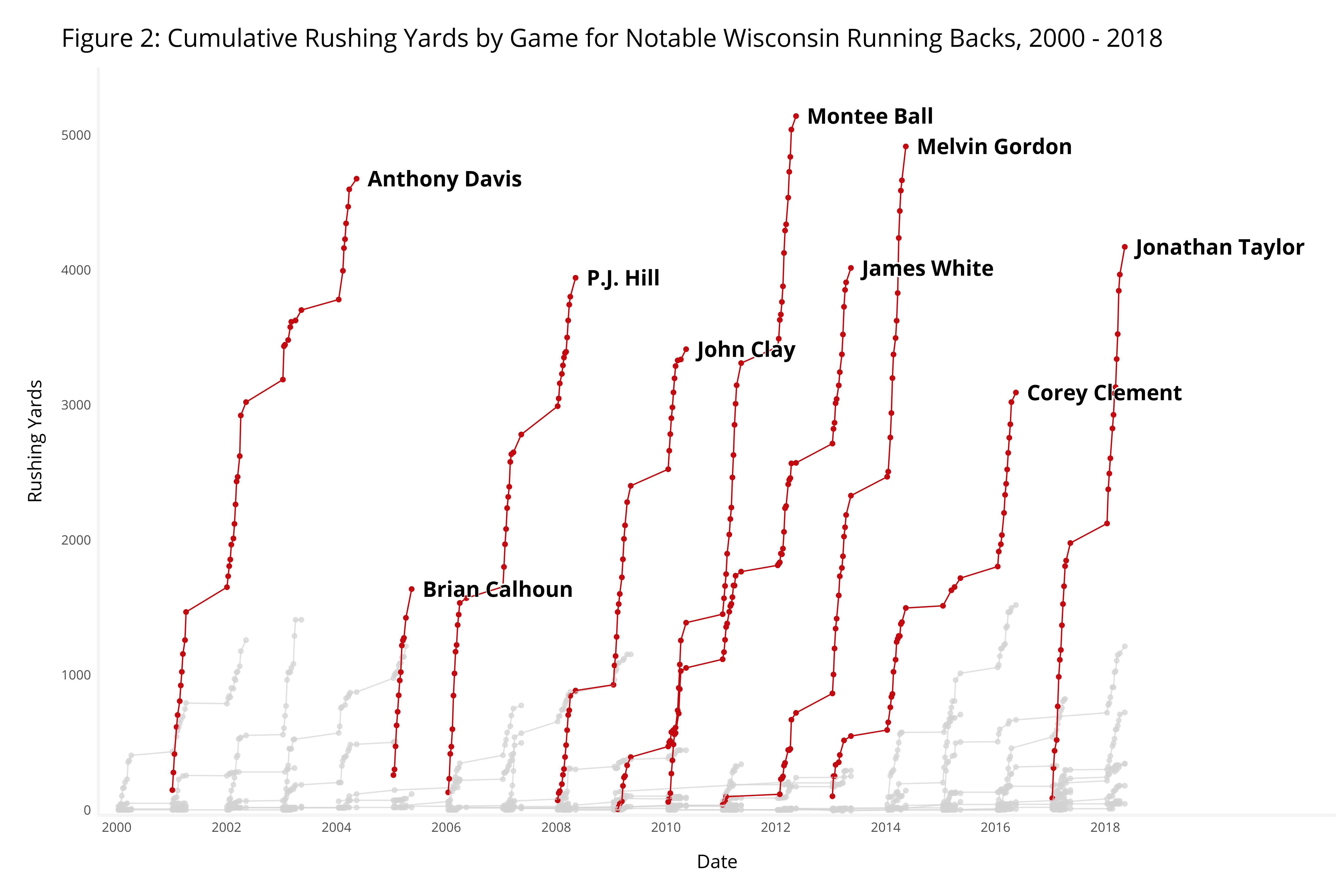
          labs(title = "Figure 2: Cumulative Rushing Yards by Game for Notable Wisconsin Running Backs, 2000 - 2018", y = "Rushing Yards",  x = "Date")

    figure3 <- ggplot() +
        geom_point(data = subset(dat, playerID %in% xx$playerID), aes(gameNo, roll_sum_yards, group = playerID), color = "lightgrey", alpha = .7) +
        geom_point(data = subset(dat, playerID %in% xx$playerID & playerID %in% leadingRushersGame), aes(gameNo, roll_sum_yards, group = playerID, color = playerID), alpha = 1) +
        geom_line(data = subset(dat, playerID %in% xx$playerID), aes(gameNo, roll_sum_yards, group = playerID), color = "lightgrey", alpha = .7) +
        geom_line(data = subset(dat, playerID %in% xx$playerID & playerID %in% leadingRushersGame), aes(gameNo, roll_sum_yards, group = playerID, color = playerID), alpha = 1) +
        geom_shadowtext(data = subset(dat, playerID %in% xx$playerID & playerID %in% leadingRushersGame) %>% group_by(Player)%>% slice(which.max(roll_sum_yards)),
                        aes(gameNo, roll_sum_yards, label = paste0("  ",Player), color = playerID), bg.colour='white', size = 6, hjust = 0, family = "Open Sans") +
        guides(color=FALSE)  + scale_x_continuous(limits = c(0,60),expand = c(0, 0)) +
        scale_y_continuous(expand = c(0, 0), limits = c(-20, 5500)) + themeWisconsin() +
        scale_color_manual(values = getPallette(length(unique(leadingRushersGame)))) +
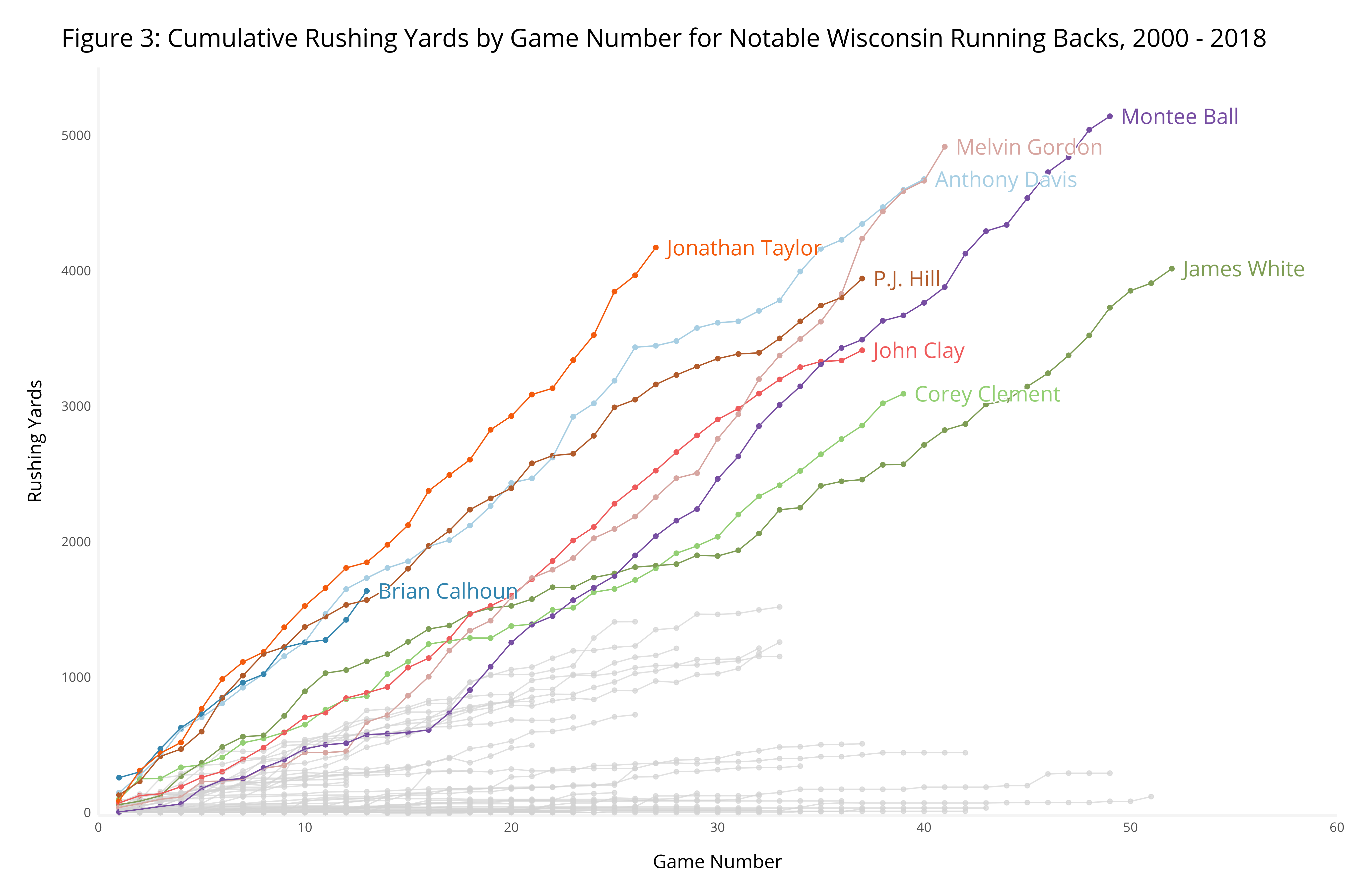
          labs(title = "Figure 3: Cumulative Rushing Yards by Game Number for Notable Wisconsin Running Backs, 2000 - 2018", y = "Rushing Yards",  x = "Game Number")

Comparing Wisconsin Running Backs Rushing Production by Seasonal Production, 1956 - 2018

    figure1 <- ggplot(data = z2, aes(season, roll_sum_yards, group = playerID)) +
        geom_point(color = "#c5050c") +
        geom_line(color = "#c5050c") +
        geom_text_repel(data = z2 %>% group_by(Player)%>% slice(which.max(roll_sum_yards)),
                        aes(season, roll_sum_yards, label = paste0("  ",Player)), color = "black", size = 6, direction = "y", family = "Open Sans", fontface = "bold", hjust= 0, segment.colour = NA, point.padding = NA) +
        guides(color=FALSE) + scale_y_continuous(expand = c(0,0), limits = c(-20, 8000)) + scale_x_continuous(limits = c(1968,2028),expand = c(0, 0)) + themeWisconsin() +
          labs(title = "Figure 1: Cumulative Rushing Yards by Season for Notable Wisconsin Running Backs, 1968 - 2018", y = "Rushing Yards",  x = "Date")


    figure4 <- ggplot() +
        geom_point(data = subset(z2, playerID %in% z2$playerID), aes(seasonNo, roll_sum_yards, group = playerID), color = "lightgrey", alpha = .7) +
        geom_point(data = subset(z2, playerID %in% z2$playerID & playerID %in% leadingRushersSeason), aes(seasonNo, roll_sum_yards, group = playerID, color = playerID), alpha = 1) +
        geom_line(data = subset(z2, playerID %in% z2$playerID), aes(seasonNo, roll_sum_yards, group = playerID), color = "lightgrey", alpha = .7) +
        geom_line(data = subset(z2, playerID %in% z2$playerID & playerID %in% leadingRushersSeason), aes(seasonNo, roll_sum_yards, group = playerID, color = playerID), alpha = 1) +
        geom_shadowtext(data = labelDat, aes(seasonNo, roll_sum_yards, label = paste0("  ",Player), color = playerID), bg.colour='white', size = 6, hjust = 0, family = "Open Sans") +
        guides(color=FALSE) + scale_x_continuous(labels=c(0:4), breaks=c(1:5),limits = c(1,6),expand = c(0, 0)) +
        scale_y_continuous(expand = c(0, 0), limits = c(-20, 8000)) +  themeWisconsin() +
        scale_color_manual(values = getPallette(length(unique(leadingRushersSeason)))) +
          labs(title = "Figure 4: Cumulative Rushing Yards for Notable Wisconsin Running Backs by Seasons in Program", y = "Rushing Yards",  x = "Season")

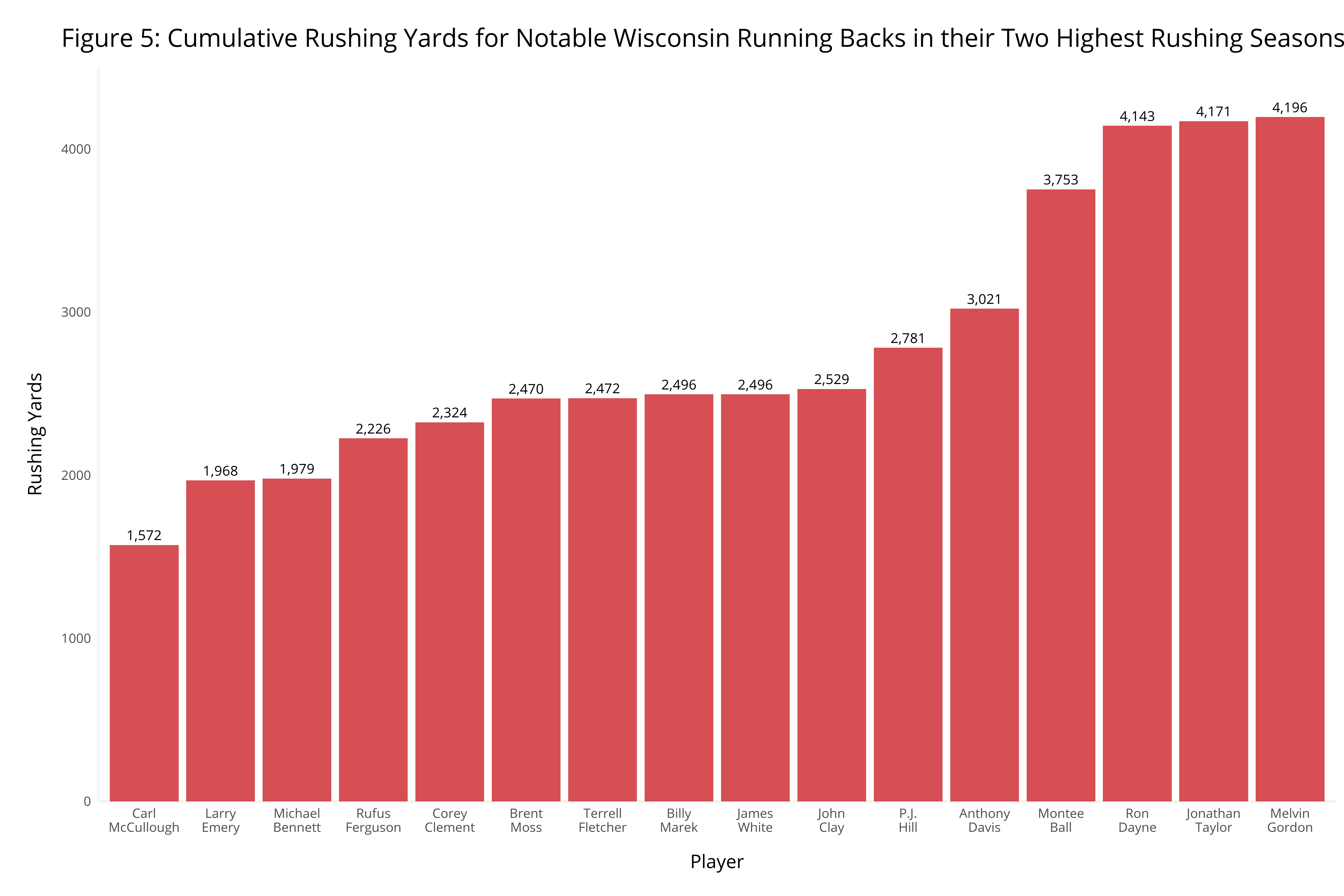
    figure5 <- ggplot() +
        geom_col(data = z5, aes(x = playerOrder, y = roll_sum_yards), fill = "#c5050c", alpha = .7) +
        scale_y_continuous(expand = c(0,0), limits = c(0,4500)) +
        geom_text(data = z5, aes(x = playerOrder, y = roll_sum_yards, label=format(z5$roll_sum_yards, nsmall=0, big.mark=",")),family = "Open Sans", vjust=-.5) +
        guides(color=FALSE) + themeWisconsin() +
        labs(title = "Figure 5: Cumulative Rushing Yards for Notable Wisconsin Running Backs in their Two Highest Rushing Seasons", y = "Rushing Yards",  x = "Player")

Wisconsin has employed an incredible sequence of successful running backs since Barry Alvarez breathed life into the program in the early 1990s. Ron Dayne, Montee Ball, Melvin Gordon, and Taylor have each finished in the top 10 of Heisman voting - Taylor doing so twice - while also winning the Doak Walker Award for the best collegiate running back.

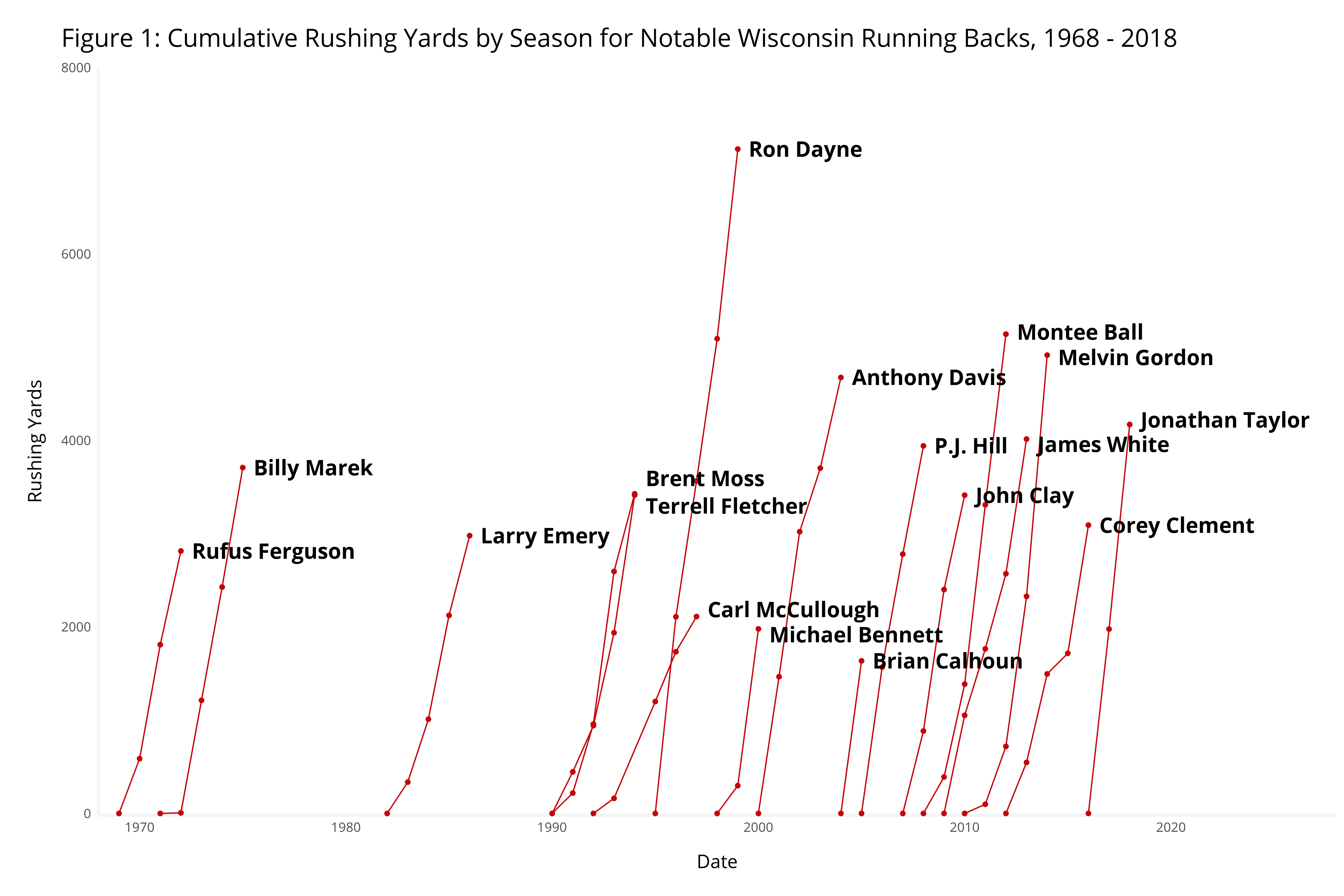
Figure 1: Cumulative Rushing Yards by Season for Notable Wisconsin Running Backs, 1968 - 2018

As displayed in Figure 1, the four-year production of Ron Dayne stands out from the recent crop of running backs. Dayne’s contributions on the field resulted in breaking the FBS career rushing mark (since eclipsed, controversially) in 1999, and he deserves some credit for establishing the class of running back commit Wisconsin is able to sign to this day.

Taylor stands on the shoulders of a legacy of elite rushing prospects. Looking more closely at single game rushing data over time in Figure 2, Taylor fits in neatly with his fellow Badgers - he is equal in stature to the best recent Wisconsin running backs. It’s incredible to reflect on the 2011 data points signifying a Wisconsin team that fielded Montee Ball, James White and Melvin Gordon (albeit for only 3 games) simultaneously!

Figure 2: Cumulative Rushing Yards by Game for Notable Wisconsin Running Backs, 2000 - 2018

When considering the rushing totals by game number is where his success has few comparisons. Figure 3 shows the cumulative rushing yards by game starting in 2000, the first year that single game data is available. Three things pop out to me:

Anthony Davis and P.J. Hill had much better careers than I recall
Brian Calhoun had a monster first game as a Badger - 258 yards rushing against Bowling Green!
James White and Montee Ball played a lot of games in their career
Jonathan Taylor’s first 27 games have been unreal

Figure 3: Cumulative Rushing Yards by Game Number for Notable Wisconsin Running Backs, 2000 - 2018

In fact, when compared to all Wisconsin rushers in their first two seasons (regardless of academic standing) Taylor’s are the most yards all time. As seen in Figure 4, it’s not particularly close!

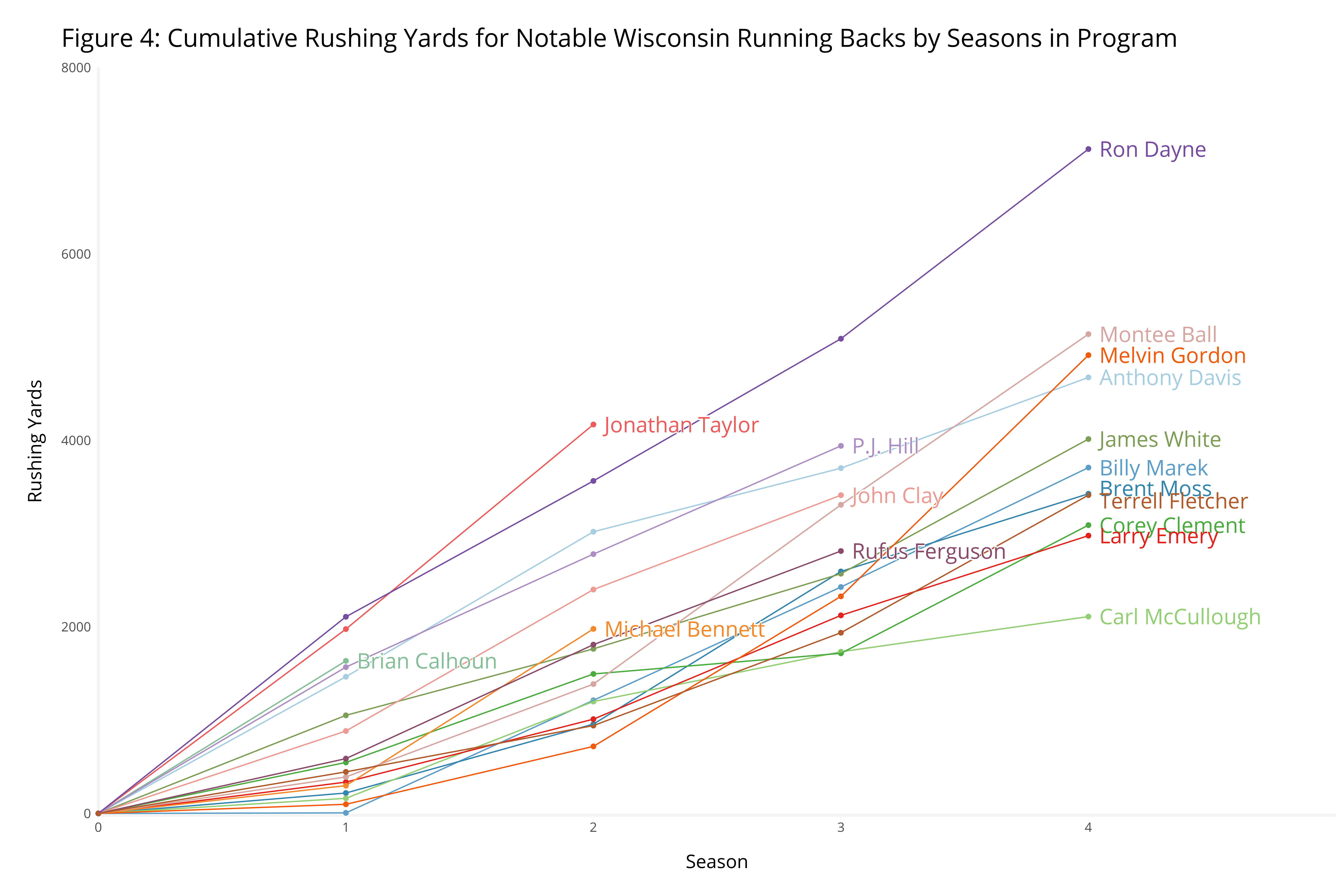
Figure 4: Cumulative Rushing Yards for Notable Wisconsin Running Backs by Seasons in Program

He is comfortably on pace to accrue more rushing yards than all Wisconsin running backs (aside from Ron Dayne) by the end of his junior season. If he returns for his senior season, the FBS career rushing mark might be in reach. Figure 5 displays the top two rushing seasons for notable Wisconsin running backs during their careers. The total rushing of Taylor’s freshman and sophomore campaigns stack up as the second highest total of the any of the two best seasons of all Wisconsin running backs.

Figure 5: Cumulative Rushing Yards for Notable Wisconsin Running Backs in their Two Highest Rushing Seasons

Over the first two seasons of his career, Taylor accumulated more rushing yards:

than any rusher in school history over their first two years
than P.J. Hill, John Clay, and Rufus Ferguson in their three college seasons
than James White, Billy Marek, Brent Moss, Terrell Fletcher, Corey Clement, Larry Emery, and Carl McCollough in their four respective college seasons

Jonathan Taylor has chewed up yards - and the best might still be to come.